Viticulture & Enology Extension News – Spring 2012

2011 Overview: The Silver Lining in Summer Clouds

By Michelle Moyer (Viticulture); Federico Casassa, PhD Candidate, and Jim Harberston (Enology), WSU Prosser

From the Vineyard

As the AgWeatherNet reports roll in regarding warmer temperatures and spring rains, it is hard to take a retrospective look at 2011 with the 2012 growing season teasing us from the not-so-distant future. We have a lot to learn from history, however, even if that history was only a few months ago.

Cool springs, prolonged bloom, and extended véraison.

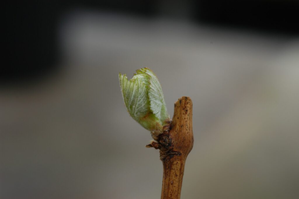
The “hot” topic of the 2011 growing season was the utter lack of summer. Fashionably late, summer did not show until August. The cool spring temperatures delayed both budbreak and flowering by 2 to 4 weeks (Fig. 1), putting the 2011 vintage behind the notoriously cool 2010 vintage on a calendar comparison. But that late arrival of heat came at the necessary time to bridge the gap between “average” development timing and the delayed timing seen last year.

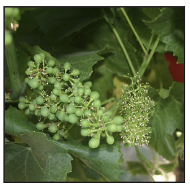
The 2011 harvest lagged behind historical average dates for most locations, however, those locations that completed bloom within in a reasonable time were still able to pick a crop. Sugars were perhaps lower than desired, and acidity initially appeared high, but this did not always translate into negative quality. Federico Casassa and Dr. Jim Harbertson discuss the outcomes of the 2011 grape vintage on wine quality in “From the Crush Pad”.

Freeze damage and retraining.

As discussed in the Fall 2011 issue of VEEN, the cool, wet spring of 2011 may have been crucial to those vineyards recovering from the Thanksgiving Freeze of 2010. In fact, many vineyards recovered at an unexpected rate, and in some cases, vine vigor translated into uncontrollable growth and inappropriate internode length for future spur positioning (Fig. 2). Why was this, and how can we learn from this situation to help prevent these retraining issues in the future?

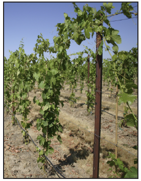
It appeared that the largest contributing factor to excessive vine vigor in retraining situations was the lack of consideration of the available nutrient reserves and capacity a vine with a well-developed root system. While the retention of one to three developing shoots may be appropriate in the establishment phase of vineyard development when the vine has a small root system, one to three developing shoots on a mature root system is simply an insufficient sink size to appropriately disperse the amount of source energy available in the spring. This root system is still approximately the same size and function as when you would leave a full complement of buds; although there is a loss of some reserves from the death of the trunk and cordons, that loss does not practically translate to reducing bud number from a “normal” full bud complement to a few trunk-base buds (and subsequent shoots). In many cases, vigor was adequately controlled by retaining ~5 base shoots, and only removing the unnecessary shoots at the end of the season, after desired shoot internode length was achieved.

Disease management.

While there were some challenges in keeping the upper hand over Powdery Mildew in 2011, there were some important lessons to be learned. First, timing is everything. This is not simply referring to getting chemical protection on during the critical period of susceptibility (immediate prebloom to 3 weeks post fruitset), but also referring to maintaining proper spray intervals, and slowing tractor driving speed. These factors are important in low-pressure years, and absolutely critical in high-pressure years. The 2011 growing season also highlighted the benefits of using such cultural practices as fruit-zone leaf removal and shoot thinning as necessary partners with chemical controls in effective management programs. While the intensity of a chemical regime for 2012 may change based on disease pressure, it would be ill-advised to downplay the fact that cultural strategies should always be used to maximize chemical effectiveness.

2012 and beyond.

While we hope for the return of “normal” conditions in 2012, let’s not forget the lessons we have learned in 2011. Challenging vintages remind us that we are fortunate to not deal with these conditions on an annual basis. However, this is not an excuse to be complacent; the information and experience gained from these vintages can be extrapolated to future vintages to improve our reactive measures, or better yet, develop proactive strategies.

From the Crush Pad

There were many publicly, and privately, exclaimed adjectives winemakers throughout the state have been using to characterize the 2011 harvest in Washington; ones which we will refrain from using. Luckily, a lot can happen from harvest to barrel, and in the process, adjectives change. We planned to divide this short report in two sections: the first will highlight the very well-known facts of the 2011 harvest, and the second highlights a few under-the-radar results of the 2011 vintage.

Facts on the 2011 Vintage

Late harvest.

As mentioned in “From the Vineyard”, harvest was 2 to 3 weeks behind. Since we had unseasonably cool and wet spring, this was expected.

Optimum photosynthesis.

August and September were almost ideal, with cool nights and only a few days surpassing the 95°F threshold of photosynthesis shutdown.

Condensed maturity.

A late and condensed maturity window posed problems in terms of harvest and winemaking logistics. Manual labor is a challenging issue Washington: when the grape harvest is late, it overlaps with apple harvest, which is by far more profitable for pickers.

Lesser-Known Facts

Berry size.

The 2011 vintage surprised many winemakers with unusually large berries, even in varieties such as Cabernet Sauvignon. For example, in one of our research vineyards, Cabernet Sauvignon berries were 18% larger than 2010, and 22% larger than those from (a warmer) 2009. Larger berry sized resulted in larger volume of juice being received than what was forecast, which in turn resulted in slight underestimation of barrel stocks and tank space needed for the 2011 harvest.

Acidity.

While most winemakers were expecting a “high acid” vintage, we observed some rather unusual behavior of the fruit acids in the transition from grapes to wine. Specifically, there was a mismatch between titratable acidity (TA) measured in the fruit, and TA measured in the must and then in final wines. On multiple occasions, acids in the fruit were lower than those in the wines, even after malolactic fermentation. Table 1 contains data from a Merlot trial, which represents this perplexing acid evolution. Initially, TA in the grapes was low, close to the levels of those in the tank sample after crush. Once fermentation was fully active (Fig. 3), TA values almost doubled in some cases. (Note: Fermentation samples should be thoroughly degassed prior analysis due to the acidic character of the dissolved CO₂).

Sampling Time	Titratable Acidity (g/L tartaric acid)
Tank sample after crush	4.27 ± 0.06
Tank sample 5 days after crush	7.82 ± 0.01
Beginning of cold-stabilization (December 2011)	7.42 ± 0.02
February 2012	6.39 ± 0.02
Bottling (March 2012)	5.10 ± 0.01

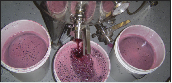
Even more striking was that wines tasted incredibly sour, far more acidic than the “natural” acidity we tasted in the tanks upon crushing. We are hypothesizing that both the skins and the pulp retained substantial amounts of acids, which were released as a result of heat, enzymatic activity, and mixing during fermentation/maceration. We plan to test this hypothesis, as it is not clear whether this phenomenon is solely a product of cool vintages.

As an aside, we found that if we followed a protocol for analyzing TA in frozen Concord grapes (heating the samples at 149°F for 1 hour), the measured acidity of the juice approached those measured at this “peak” of TA and pH. Many winemakers have described issues with measuring acidity and have normally attributed these issues to sampling. It is possible that the heating procedure may improve TA estimates.

Chaptalization.

Although statewide generalizations cannot be made, chaptalization in late ripening varieties such as Sangiovese, Carmenere and Petit Verdot in some cooler AVAs occurred.

Tartaric acid stabilization.

There were some issues in both red and white wines upon cold stabilization; instability led to light cloudiness in some wines. The haze did not seem to have any detrimental effect on the wines, other than the visual appeal. The haze appeared to be colloidal in nature, and filtration through a 0.45 µm membrane filter with an electrically neutral membrane polymer failed to remove the haze. However, after filtering the wine through a charged medium (e.g. cellulose esters) the haze was successfully removed. This haze was also easily removed by centrifugation in the laboratory (14,000 rpm). Based on our observations we think this colloid involves organic acids.

2012 and beyond.

While we felt that 2010 was a cool vintage, 2011 provided several new challenges. Despite this, the overall quality for the wines made here in Prosser was quite high. However, we too are hoping for a warmer 2012!

USDA Plant Hardiness Zone Map Updated

By Michelle Moyer, WSU Prosser

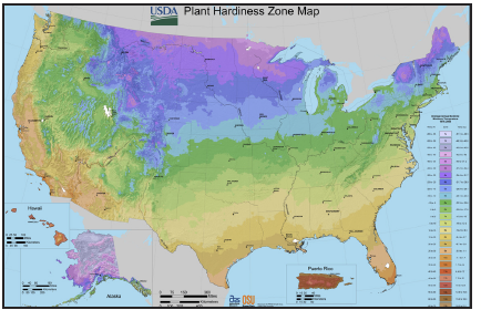
The USDA-ARS has released an updated Plant Hardiness Zone Map. The information presented in the map can be used to assess if different plant species, and varieties, will thrive at your site or suffer routine dieback due to freeze damage.

For grape growers, they are a great initial information source in determining if a site is suitable (i.e. winters are not too cold) for grape production, and which species (Vitis vinifera, V. labrusca, or various hybrids) would be the most appropriate given winter temperature limitations.

Plant hardiness zones are constructed using the average of the annual extreme low winter temperatures (i.e. the coldest temperature recorded that year) over a 30 year period. If your location has changed ratings, please keep the following in mind: While these average absolute low temperatures do provide a guide as to whether a plant will survive a location’s winter on a routine basis, the occurrence of extreme low temperature events can still limit production. These extreme weather events are not always apparent in averages.

For example, if the extreme low temperatures for a given site over five years were: 8ºF, -2ºF, -7ºF, -15ºF, 0ºF, the average would be -3.2ºF.

For V. vinifera this is an appropriate average low temperature (Zone 6b), but that one in five year event of -15ºF could result in substantial cold damage (of course, this is moderated by the timing of the extreme cold temperature event relative to vine cold hardiness acclimation).

Maps can be downloaded from the website, or the new interactive interface can be used down to zip-code specific zone information.

Unlike past editions, posters of the maps have not been printed, but the download options from the USDA website allow you to print them in a variety of size options.

Mealybug Pheromone Traps: How Many Do You Need?

By Brian Bahder, PhD Candidate, WSU Prosser

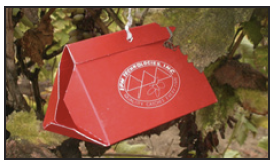
The sex pheromone for the grape mealybug was recently synthesized and is now commercially available for implementation in monitoring programs. This pheromone (trans-alpha-Necrodyl isobutyrate) attracts the adult male mealybug. Their presence or absence in a vineyard can be used as a proxy for the female grape mealybug.

This method of capture and monitoring provides a faster and more economical means to monitor for the presence of the grape mealybug. The traps are also commercially available, making them easy to obtain.

Trials were conducted at WSU-IAREC in Prosser, WA in 2009, 2010, and 2011 to determine the optimal trap density (number of traps needed in a vineyard bock) to effectively monitor for the grape mealybug. Trap densities of one, four, and eight traps per 30 acres were tested in Concord and Vitis vinifera vineyards in the Prosser and Paterson area.

Weekly trap data (number of adult males per trap) were collected over the course of the growing season. Results from 2010 are seen in Figure 1. Adult male mealybugs started to fly around the beginning of May, and peak flight activity occurred in the middle to end of June. After a few weeks, a second flight occurred, and peaked around mid to late August (Figure 1). Adult male flying activity appeared to cease at the end of October.

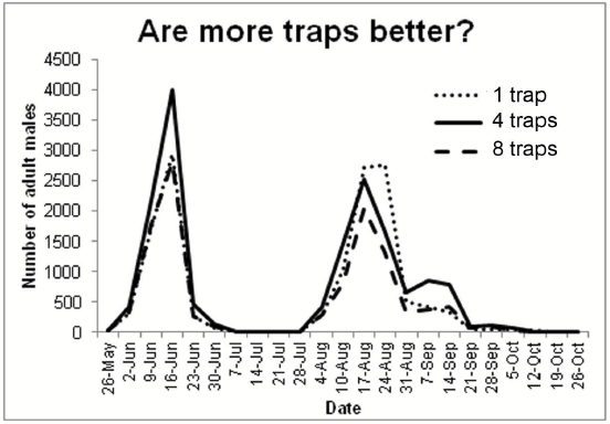
As expected, more adult males were collected overall when trap density was at 8 traps per 30 acres, versus 4 traps or 1 trap per 30 acres. This is likely the result of simply having more available traps in the vineyard, considering the average number of adult males per trap was not significantly different across the different trap density treatments. The take-home message: There is no economic incentive to placing more than one trap in a 30 acre swath of vineyard!

Why is knowing when adults emerge and fly important? Their flight pattern can be used as a measure of when early instars are present, and this is a critical stage for chemical intervention. Adult females are not susceptible to insecticides, so applications need to be made when there are young.

Monitoring of grape mealybug flight patterns will continue through 2012 to ensure previous observations are annually consistent.

Drosophila suzukii: No Longer Code Red for Washington Grapes

By Luz Denia Barrantes-Barrantes and Doug Walsh, WSU Prosser

In 2010, the threat of Drosophila suzukii (formerly Spotted Wing Drosophila) was an important concern for soft fruit growers. As a part of the monitoring process for this new, invasive pest, a second year of monitoring was conducted in Benton and Franklin counties in 2011.

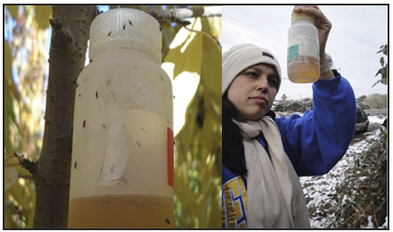
Nine crops were selected (Table 1) for monitoring in 2011, due to previous reports identifying them as potential hosts of D. suzukii. A total of 180 traps were placed in the crops with a minimum distance of four meters between each trap (Figure 1). Two trap types were used: apple cider vinegar (ACV; 126 traps), and fermenting yeast (yeast, sugar, and water; 54 traps). Traps were checked biweekly from March to May, and weekly from June to November.

Crop	Number of Traps
Apple	6
Apricot	8
Blackberry	30
Blackberry/Raspberry*	4
Blueberry	35
Cherry	17
Juice grapes	46
Peach	10

Bait Recipes

Apple Cider Vinegar: Add 3 oz of natural flavor apple cider vinegar (5% acidity) and 3 drops of liquid dish detergent to your trap.

Fermenting Yeast: Mix 1/3 cup dry active yeast, 2/3 cup of sugar, 1 gal of water and 3 drops liquid dish detergent. Place 3 oz of this mixture in your trap.

Results

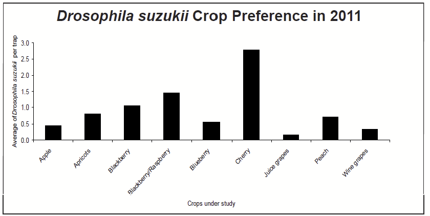
Cherries were by far the most attractive for D. suzukii (averaging 2.78 flies per trap), followed by blackberries/raspberries (1.45 flies per trap). Fortunately, for grape growers in WA, it appeared that D. suzukii has low overall preference for both juice and wine grapes (Figure 2). Concord grapes were not highly favored (0.15 flies per trap), with only a slight increase in preference for wine grapes (0.34). This was despite having a high concentration of traps in these two crops (25% of the total traps in Concord, and 13% of the total traps in wine grapes). This strengthens the argument that grapes appear to be a non-preferential crop for D. suzukii.

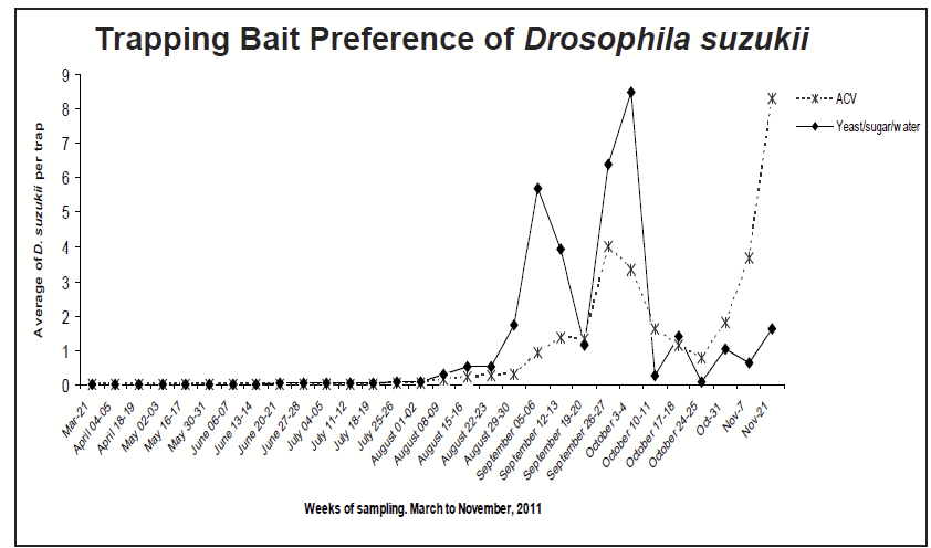
When comparing the bait types (ACV vs. fermenting yeast), flies appeared to prefer the fermenting yeast (1.13 flies per trap) over the ACV (0.97 flies per trap) (Figure 3). The effectiveness of the bait appears to be related with the ambient temperature. When the temperatures are moderate (>68°F) the flies are more attracted to the mixture of yeast, water, and sugar. When temperatures cooled, the apple cider vinegar is the most attractive bait (Figure 3).

Recommendations

Although monitoring and other reports suggest that D. suzukii will likely not become a major pest in grapes, it is important to practice timely harvest.

If you have damaged or infested fruit, remove it from the vineyard and destroy it. We have low infestation in grapes, so let’s keep it that way!

If you want to do your own monitoring, use ACV bait during the months where the average temperature is lower than 68°F and fermenting yeast during warmer months.

Irrigation Scheduling for (Wireless) Washington

By Troy Peters, WSU Prosser

It is irrigation season, once again! This brings up age-old questions such as: “When do I turn the water on?” and “How long do I leave water on?”

Improved irrigation scheduling has tremendous public and private benefits including better yields, improved crop quality, lower pumping energy costs, lower labor costs, and decreased loss of costly fertilizers due to leaching. While a variety of irrigation scheduling aids are available, they are not widely used and most of them are not adapted to Washington. The common reasons behind their lack of adoption are: (i) they are too complicated, (ii) they are difficult to learn, and (iii) they are time consuming to use. In addition, growers rarely have time, or desire, to complete the associated “desk-work.”

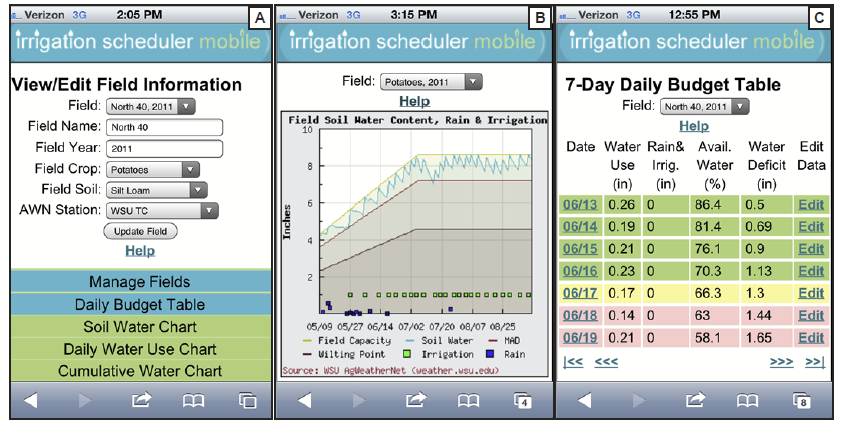
To fill this need, Washington State University has developed a simple, user-friendly, and mobile irrigation scheduling tool. Irrigation Scheduler Mobile is a free irrigation scheduling tool for doing simplified check-book style irrigation scheduling that is designed for use on a smart phone or desktop web browser. It is easy to set up and automatically pulls daily crop water use (evapotranspiration) estimates from WSU’s AgWeatherNet (AWN; weather.wsu.edu). It also allows modifications for improved accuracy by users. The model can be corrected at any time using soil water measurements or estimates. It readily displays useful charts and tables for visual evaluation of soil water status and model inputs.

After logging in, users can define specific setting for individual field sites (Figure 1a). This involves: (i) Naming the field site (e.g. Joe’s Cab Vineyard), (ii) Selecting the year, (iii) Selecting the crop grown, (iv) Selecting the soil texture, and (v) Selecting the AWN weather station that is closest to their site.

Based on these inputs, that particular field site is then set up with default values for the soil’s water holding capacity and average crop growth characteristics. Rainfall and daily crop water use estimates are imported from the associated AWN weather station.

The soil water content is shown on the Soil Water Chart (Figure 1b) along with the maximum amount of water that the soil can hold (field capacity), the wilting point, and the point where the plant will begin to see water stress (also called the management allowed deficit , or MAD). For maximum growth and production, the soil water content should be maintained between the field capacity and MAD. To induced stress, the soil water content should be maintained somewhere underneath MAD, but above the wilting point.

From the Daily Budget Table (Figure 1c) the user can see the soil water deficit (maximum amount of water that can be added without losing it past the root zone) and edit the rainfall and irrigation amounts. In addition, the user can correct the soil water content using on-site soil moisture measurements or estimates.

The model accuracy can be improved by revising the default soil and crop growth parameters and dates in the Advanced Field Settings. A complete user’s manual is available online and a full screen version that runs within AWN will soon be released. The Irrigation Scheduler Mobile is available at: http://weather.wsu.edu/is/

For more information, contact Troy Peters at troy_peters@wsu.edu.

Evaluation of Tannin Additives to Red Wine

By Jim Harbertson, WSU-IAREC and Mark Downey, DPI-Victoria, Australia

Tannins are an important part of wine quality and are frequently added during winemaking. Tannins are added to wine for a range of reasons including effecting the sensory properties of the wine, deactivating enzymes, or bolstering the amount of antioxidants. Tannin additives, also referred to as enological tannins, and their impact on wine are poorly documented, however, their use during fermentation and cellaring is widespread in the wine industry.

In collaboration with Chateau Ste. Michelle, scientists from DPI-Victoria (Australia), UC-Davis, and WSU sought to characterize a range of enological tannins and their contribution to wine quality. Numerous enological tannins were surveyed for protein precipitable tannins and iron reactive phenolics. In general, the enological tannin products were relatively impure, ranging from 12 to 48% tannin.

In this same study, one enological tannin product, which was a mixture of grape and oak tannins, was added to a Merlot wine during barrel ageing, at various concentrations ranging from 60 to 300 mg/L. Interestingly, only the 300 mg/L addition had a significant increase in measurable tannins in the final wine product.

Given the impurity of the enological tannin products, it was not surprising that no differences between the control and treated wines were observed. This prompted a second experiment that greatly increased the amount of enological tannin addition to wine.

In the second experiment, grape (condensed) and oak (hydrolyzable) enological tannins were added to Cabernet Sauvignon wine post-pressing at recommended (150-200 mg/L) and high (600-800 mg/L) rates. Wines were analyzed for anthocyanin, small and large polymeric pigment, precipitable tannin, iron reactive phenolics and sensory character.

Following all enological tannin additions, tannins were readily measured in the wines and were discriminated in sensory analysis with higher brown color, bitterness, and earthy character. Other parameters were rated with lower intensity. The initial red wine had ~550 mg/L tannins, which is about average for all red wines, while the additions increased the wine tannin from 50 to 250 mg/L.

Generally, the recommended addition rates by tannin manufactures were too low to impact the measured tannin concentration of Merlot and Cabernet Sauvignon wines from Washington (USA). The oak- and grape-based enological tannin additions had a measurable impact on wines, but unfortunately, they also had a negative impact on sensory character.

In conclusion, enological tannins are added to wines for a range of reasons. This research suggests many enological tannin additions may be unjustified and have limited or negative impacts on wine quality.

Maceration Part 2: Focus on Color

By Federico Casassa (PhD Student) and Jim Harbertson, WSU Prosser

The color of red wine has always been at the heart of human fascination, and this holds true for both scientists and winemakers.

Raymond Brouillard, a world-renowned phenolic chemist who resolved the structure of several anthocyanins in flowers, fruits and legumes was amazed by the fact that even though the structure of grape anthocyanins is among the simplest encountered in higher plants, the color of red wine is more stable than the color of other anthocyanin-based food products (1). Why is this so?

Raymound Brouillard proposed that the structural simplicity of grape anthocyanins and the lasting color of red wine should be considered as “The French Paradox II”.

An intriguing aspect of red wine color that has been recently demonstrated is that more skin contact time during maceration does not necessarily result in more immediate color (2). While the final color of red wine is highly dependent on the grape variety, there are intrinsic aspects of the winemaking process, such as skin contact time, that modulate how color is extracted.

Color evolution during maceration.

As shown in Figure 1, the wine made with a skin contact time of 4 hours is pink in color. This wine is, for all practical purposes, a rosé wine presumably devoid of structure and mouthfeel due to the minimal or non-existent extraction of tannins. Within 48 to 96 hours, the maximum color of the wine is attained. Color seems to remain stable thereafter, as evidenced by the spectrum of the 8-day wine, which does not differ from the 96-hour wine.

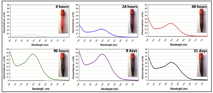
A snapshot of the maceration process in a Malbec wine made on an industrial scale and using different skin contact regimes (4 hours to 21 days), is seen in Figure 1. The insets are the actual appearance of the finished wines. The spectra show which color wavelengths are absorbed in the visible range of the electromagnetic spectrum. A maximum peak of absorbance at 520 nm corresponds to the absorption of red light and this is the dominant color spectrum in red wines. In fact, anthocyanins strongly absorb light at 520 nm, a physical-chemical trait that is used for their quantification. On the other hand, the more “lifted” or “flat” the spectrum is, the more or less “visible” color the wine displays, respectively.

Beyond 96 hours, however, other compounds such as tannins are extracted thus contributing to the mouthfeel of the wine. The same holds true for the 8-day wine. Finally, the spectrum of the 21-day skin contact time wine is more “flat” than the spectrum of the 96-hour wine. The conclusion is obvious: the 21-day maceration wine has less color than its 96-hour or 8-day maceration counterparts.

How can this be? It has to do with the nature of the anthocyanins. During post-fermentation, a decrease in the concentration of anthocyanins is typically observed. This apparent loss is the result of the combined effects of degradation reactions (mainly non-enzymatic oxidations), electrostatic binding (3), and to the incorporation of the anthocyanins into a new family of pigments dubbed “polymeric pigments” (4,5).

Are we really losing color? The answer is yes, at least in the short term. This is the rationale followed by winemakers who macerate for 5-7 days, in order to obtain deeply colored, young red wines, which are designed to be consumed quickly. The interesting part is what happens in the long term. While a 21-day maceration results in a wine with lower color density than a 96-hour maceration, it contains something that its 96 hour counterpart does not: tannins.

Although not directly verifiable in the short term, it is likely the 21-day maceration wine will develop a more stable color due to the progressive formation of polymeric pigments.

Polymeric pigments explain the high stability of red wine color.

Polymeric pigments are a heterogeneous mixture of monomeric, oligomeric and polymeric tannins that have an anthocyanin attached to it (Figure 2d).

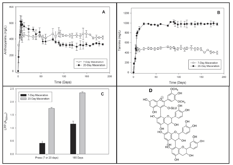
By virtue of the glucose moiety of the anthocyanin portion, they are water-soluble and are less astringent than the intact, original tannin (4) Moreover, unlike anthocyanins, polymeric pigments tend to be more resistant to pH changes, temperature and bisulfite bleaching (3) (all aspects normally encountered during winemaking), which renders them more stable. In fact, one of the virtues of extended maceration may be the gain of more stable color together with a modulation of the astringent properties of the tannins as a result of enhanced polymeric pigment formation (2).

Conclusion

Red wine color is complex and much research is still devoted to understand the biochemical basis of its development and evolution during winemaking. From the perspective of color, maceration is a trade-off: with longer maceration times, more tannins are extracted but this is at the expense of some loss of anthocyanins (Figure 2a-c). However, the anthocyanins that remain are likely to persist longer in the wine matrix, and might soften the astringency of red wine as they become progressively incorporated into polymeric pigments.

References

1. Brouillard, R., Chassaing, S. and A. Fougerousse. Phytochemistry, 64:1179-1186.
2. Casassa, L.F., M. Mireles, E. Harwood and J. F. Harbertson. 2011. American Society for Enology and Viticulture Annual Meeting. Grape and Wine phenolics Technical Abstracts. 70 pp.
3. Cheynier, V., M. Dueñas-Paton, E. Salas, C. Maury, J.M. Souquet, P. Sarni-Manchado, and H. Fulcrand. 2006. Am. J. Enol. Vit. 57:298-305.
4. Haslam, E. 1998. Practical polyphenolics – From structure to molecular recognition and physiological action. Cambridge University Press, Cambridge, UK, 422 pp.
5. Harbertson, J.F., M. Mireles, E. Harwood, K.M. Weller, and C.F. Ross. 2009. Am. J. Enol. Vit. 60:450-460.