Viticulture & Enology Extension News – Spring 2016

6 Steps to Calibrate & Optimize Airblast Sprayers

By Gwen Hoheisel, WSU Regional Extension Specialist

The idea behind any pesticide application is to get every drop to the crop. Spray or drift that goes into the air clearly missed the target. This leads not only to negative environmental and health effects, but also wasted money. Pesticide applications are one of the most frequent operations carried out in the vineyard, and chemical control costs for a single spray can range from $40 to > $100/acre. So any waste, or improvement, can have a significant economic impact.

This article discusses 6 Steps for sprayer calibration and optimization. However, these assume proper maintenance and operation of the sprayer, and that the mechanical parts of a sprayer—like the hoses, pressure gauges, pumps, and agitators—are working properly.

Optimizing spray applications will take an investment in time initially, but will pay off with reduced loss and improved pest control.

Step 1. Check Speed

Speedometers on tractors are notoriously inaccurate. Being able to know your true tractor speed is important because it is used in the subsequent calibration steps and effects spray coverage. Always check tractor speed while in the field as opposed to while on a gravel road, since the terrain influences speed. There are two ways to assess speed.

Method 1: Manual Check.

In the vineyard, mark a 100 ft path with two stakes. With a stopwatch, record the time it takes for the front tire of the tractor to pass from one stake to the next. Use this formula to check the speed:

Other distances (e.g., 88 or 200 ft) can be used for the path. Longer paths, over more terrain, could eliminate some variation in time due to hills or dips. Creating 2 to 3 paths also eliminates variation. If three 100 ft paths are timed, simply take the average of all times and then calculate miles/hour.

Method 2: Use a Tool.

GPS technology can give an accurate assessment of speed. Options include purchasing a GPS unit from a local spray manufacturer or using a hiking/biking GPS device or mobile phone app. Hiking or biking apps allow for better resolution at low speeds (e.g., 3.2 mph). Additionally, many of these tools have an option to map the route and rows sprayed.

In the vineyard, start the GPS or app. Set a desired gear and throttle with the PTO on. Drive down a row for 20-30 seconds and look at the speed. If needed, change gears to obtain the desired speed, each time allowing 20-30 seconds for a proper reading on the GPS.

Step 2. Adjust the Direction of the Air

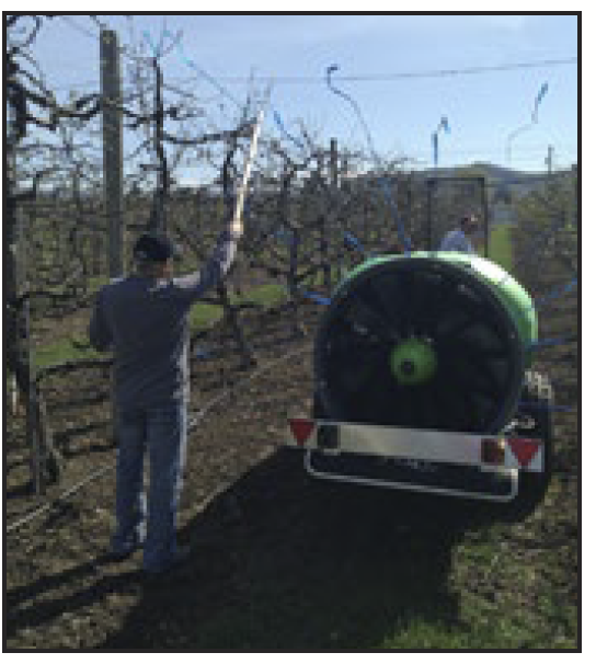
Air carries the spray droplets, meaning wherever air goes, droplets will follow. Therefore, it is critical to direct the air into the canopy or adjust for air that cannot be re-directed. Using flagging tape is a fast and inexpensive way to see the direction of air flow.

Park the sprayer in the row.

Tie flagging tape (~2 ft) to every other nozzle body and clip onto the ends of deflectors (if present). Flagging tape can also be tied to the end of a stick to extend the visualization.

Turn on the air without the spray. The flagging tape should orient just over and just beneath the canopy (Fig. 1). Use deflectors to aim air into the canopy. Consider turning off nozzles if they are not spraying into the canopies.

This optimization should be performed for EACH block with a significantly different canopy shape. Record which nozzles and deflector orientation are used for each block.

Step 3. Match the Air Volume and Speed to the Canopy

Spray should penetrate the canopy but not over-expel from the other side. Many factors like wind, canopy density, and tractor speed will affect the air volume. Ideally, there should be an automated method to adjust the air volume as conditions change.

However, significant improvements can still be seen with manual adjustments done a couple times a season depending on crop growth. Follow the steps below for 1-2 years, to determine appropriate air adjustments in the future.

1. Tie flagging tape to the top, middle, and bottom zones of the far side of the canopy from where the sprayer is driving.
2. Have one person stand at the end of the row to watch flagging tape orientation. Drive the tractor down the row using typical sprayer settings.
3. Adjust the air volume sprayer according to the results:
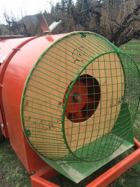
   • If the flagging blew straight out, there is too much air (common in early season). Reduce fan gear from high to low, use a plywood “donut” (Fig. 2) or a cloth shroud around the sides of the fan cage, drive faster, or gear up and throttle down (not a good option for hills).
   • If the flagging didn’t move, there is too little air. Solutions: drive slower, increase rpm or fan gear.

Note on Deflectors

The rotation of any fan, whether on an airblast or multi-fan tower sprayers, has a different air pattern on the right versus left side. As a fan rotates in a clockwise fashion air is pushed down on the right and lifted up on the left. Reverse this for fans that rotate counter-clockwise. Bottom and top deflectors can help even the airflow between the two sides. Many airblast sprayers are missing or have too short of a deflector. Many were removed because they hit fruit, but in vineyards with narrow VSP canopies, they may be useful without interfering in the canopy.

Step 4. Calculate and Record the Expected Nozzle Output

Now that the correct nozzles are used to match the air direction with the canopy shape (step 2), the gallons/minute for each nozzle can be calculated. You will need to know the running pressure in PSI and the desired gallons/acre (GPA). There are two methods that can be used calculate nozzle output.

Method 1: Manually Calculate.

Use the formula below to calculate the gallons per minute (GPM) for the entire sprayer.

GPM for each side = (GPA x mph x row width in feet) / 990

If the output from every nozzle on one side is supposed to be the same, divide the GPM per side by the number of nozzles on a side (e.g., GPM per side/# nozzles per side = output per nozzle). If output is different for each nozzle location, than the total output per nozzle must add to the GPM per side.

The output from each nozzle should be proportional to the target canopy density. A modified VSP canopy, with a narrow fruiting zone and loose shoots at the top may need 65% of the volume coming from the upper 2/3 of the nozzles, and 35% of the volume coming from the lower 1/3 of the nozzles.

For this VSP example if there are 5 nozzles open with a desired 3 GPM per side, then the upper 3 nozzles should put out 65% of the spray (1.95 GPM or 0.65 GPM for each nozzle), and the lower two nozzles should put out 35% of the spray (1.05 GPM or 0.53 GPM for each nozzle). Adjustments on volume per nozzle can be made after step 6 when spray coverage is assessed.

Lastly, look in a nozzle catalog to determine the expected nozzle output in GPM for each nozzle. For disc-core nozzles, go across the top of the table to the desired operating pressure, then go down the column to find the closest output per nozzle. Last, move left along the row to see the appropriate disc-core.

Method 2: Use an App or Software

Mobile phone apps (e.g., VineTech), Web software (e.g., Turbomist Program), and many Crop Consultant companies will calculate the total expected output for each nozzle and suggest the proper disc core. Some of the software programs also account for different canopy shapes and adjust nozzle output based on canopy density as describe in ‘Method 1’. These are great alternatives that limit manual calculations and allow for quick adjustments.

Regardless of method used, the desired output per nozzle and disc-core should be recorded.

Step 5. Measure Nozzle Output

This step can be conducted at any time to assess for worn nozzles, but it should be conducted at least once before the season begins.

1. Confirm the pressure gauge is at the correct PSI.
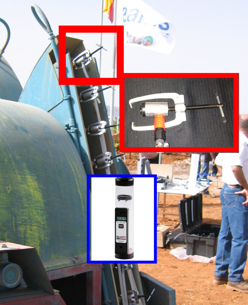
2. Connect hoses to the nozzles. Clamps that securely fit around the nozzles can be made or purchased from AAMS (Fig. 3).
3. Turn on the sprayer with water flowing. Collect the output for 60 seconds into a graduated cylinder marked with ounces. Then calculate GPM per nozzle = ounces per nozzle/128. Alternatively, use a flow meter to quickly measure output in GPM and eliminate the math.
4. Any nozzle that is more than 10% off from expected should be replaced. Replace ALL nozzles if more than 2 are bad.

Step 6. Verify Coverage

Now that nozzle orientation, air volume, and spray output are correct, you can confirm your coverage with water sensitive paper (WSP). WSP is yellow paper that turns blue with water droplets (Fig. 4). When working with WSP, always wear nitrile gloves as the moisture in your hands turns the card blue.

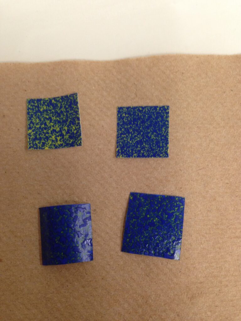
A 2-in x 3-in card can be cut into 4 to 6 smaller squares. These can be stapled to the top, middle, bottom, inner, and outer leaves of the canopy, or any other place you would like to evaluate coverage in. In addition, staple or tape WSP to 3, 1-in. x 2-in. board that is 2 to 4-ft long. These boards can be placed on the ground in the first, second and third row opposite the sprayer to determine how much spray drifted through the canopy on to the row middle.

Operate the sprayer at the calibrated settings from the previous steps and drive past the vines with the WSP. After 15 minutes (to allow the water to dry), look at the WSP to assess coverage.

The ideal spray coverage has many fine droplets all over the card without any long streaks of all blue. Areas with all blue mean too much water is being applied which leads to waste and material running-off the leaves.
Make adjustments to the sprayer or nozzle output based on your results. For example, if the spray card is completely blue in the bottom of the canopy, but few drops in the upper canopy, then either adjust the output of the nozzles or angle the nozzles differently to put more in the upper canopy. Alternatively if all the cards are blue including those on the ground, consider reducing your air volume and liquid spray volume.

Pacific Spider Mite Present in Some WA Vineyards

By David James, WSU Prosser

A survey of mites on wine grapes in Washington during 2013 to 2015 provided some interesting results. The most startling find was that California’s number one spider mite pest of grapes, the Pacific Spider Mite (Tetranychus pacificus), has been confirmed as present in some of WA’s vineyards. Confirmation of the presence of this species in Washington grapes has come from two spider mite taxonomists in Canada and Florida who have identified samples we sent to them last fall.

From the beginning of wine grape cultivation in eastern Washington, we have had two problem spider mites, Twospotted spider mite (Tetranychus urticae) and McDaniel’s spider mite (Tetranychus mcdanieli). McDaniel’s spider mite has been the dominant species. It now looks like many of the infestations thought to be McDaniel’s are in fact Pacific Spider Mite. The two species are very similar and can only be separated by examination of their genitalia (try doing that with a hand-lens!).

So what is the significance of this find of Pacific Spider Mite in Washington wine grape vineyards? We are not sure at this point. The economic impact of Pacific Spider Mite may be similar to McDaniel’s Mite and Twospotted Mite.

Spider mites generally occur in high, damaging densities on grapes under hot, dry conditions (Fig. 1) but there may be differences between the three species in this response. Spider mite populations are also exacerbated by the use of certain broad-spectrum insecticides as well as imidacloprid. But again, there may be differences between species.

We also need to know the identity of our pests for regulatory reasons and to optimize our integrated pest management programs. So the news of Pacific Spider Mite being a new addition to our grape pest fauna in Washington is not insignificant.

We currently have no idea of the extent of Pacific Spider Mite within our state and whether it’s a recent arrival or has been here undetected for some time. Interestingly, Pacific Spider Mite within California has become a bigger problem in recent years by establishing in more northern and coastal wine grape areas where it formerly was not a problem. Its impact within its traditional range has also increased. Clearly, it would be a good idea to establish the distribution of Pacific Spider Mites within our state. as well as its abundance in comparison to McDaniel’s and Twospotted Spider Mites.

The arrival of Pacific Spider Mite in Washington wine grape vineyards means that we now have four spider mite pest species. Aside from McDaniel’s and Twospotted, we also have Willamette Spider Mite which was also discovered for the first time during this same mite survey. Our survey also showed that few wine grape vineyards experienced damaging populations of spider mites but those that did were most often caused by Willamette Spider Mite. A relationship between frequent use of neonicotinoid insecticides and Willamette Spider Mite outbreaks was also suggested.

A more complex pest mite fauna in our vineyards is not necessarily a bad thing but it is certainly a situation that requires a better understanding of the roles each species plays in the potential for spider mite damage.

Phosphorous Fertilizer Management for Wine Grapes

By Joan Davenport and Catherine Jones, WSU Prosser

Phosphorus (P) is an essential plant nutrient, which means that it is required by all plants so that they can complete a full life cycle [1,3]. Phosphorus has two principal roles in the plant. It is the backbone of genetic material and also is part of the plant’s energy relations as a key element in electron transport compounds. It is very mobile in the plant, but immobile in the soil. Its high mobility in the plant explains why nutrient deficiency symptoms for P show up in the lowest (oldest) leaves first [3].

Phosphorous is referred to as a plant macronutrient because it is needed in relatively large quantities. You may have noticed when reading your annual tissue tests that P, like other macronutrients, is read as a percentage of the tissue, rather than in parts per million (ppm), the units used for micronutrients.

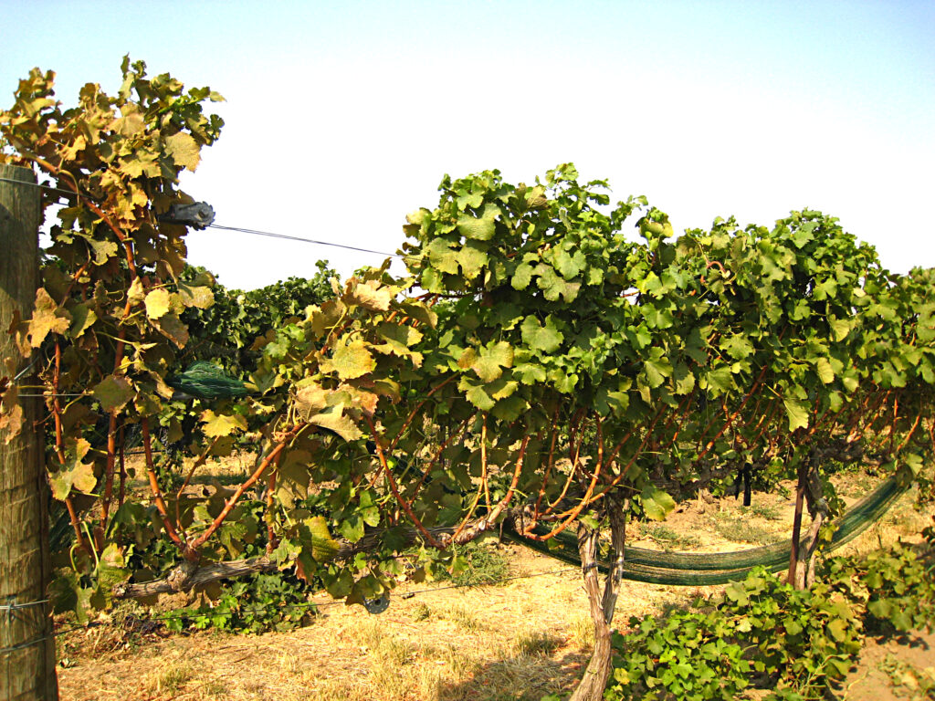
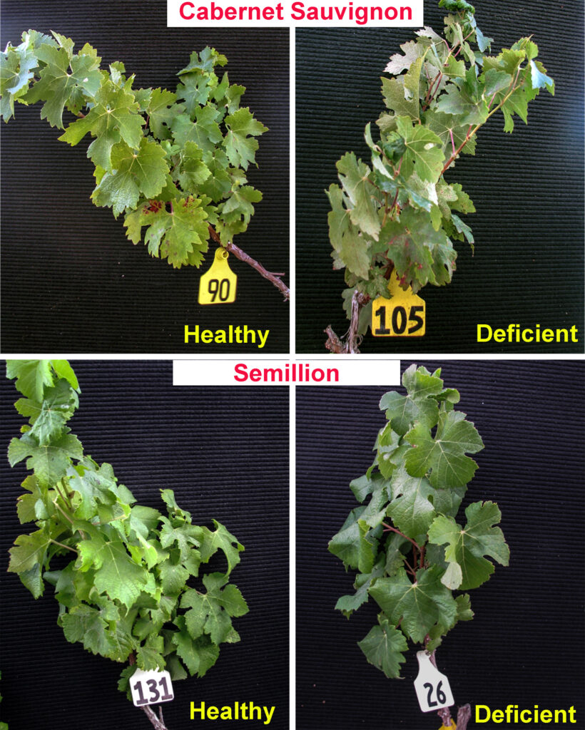
In wine grapes, low P shows up as a red discoloration in the older leaves of red varieties and a slightly darker green color in the older leaves of white varieties (Fig. 1).

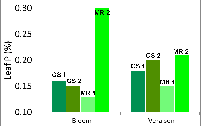
The frequency of low P symptoms has increased in the last few years. To investigate ways of relieving these symptoms, we conducted an experiment in four vineyards on the Horse Heaven Hills. The experiment was conducted in 2014 and 2015 and evaluated different rates and application types of P fertilizer and subsequent tissue leaves of P. There were two Cabernet Sauvignon (CS) vineyard blocks, and two Merlot (MR) vineyard blocks.

For two years prior to the experiment, we evaluated soil and tissue samples in each of these blocks for P. Two blocks, CS 2 and MR 1, had leaf P at bloom that were at levels considered deficient (Fig. 2), which is equal to or less than 0.15% [2].

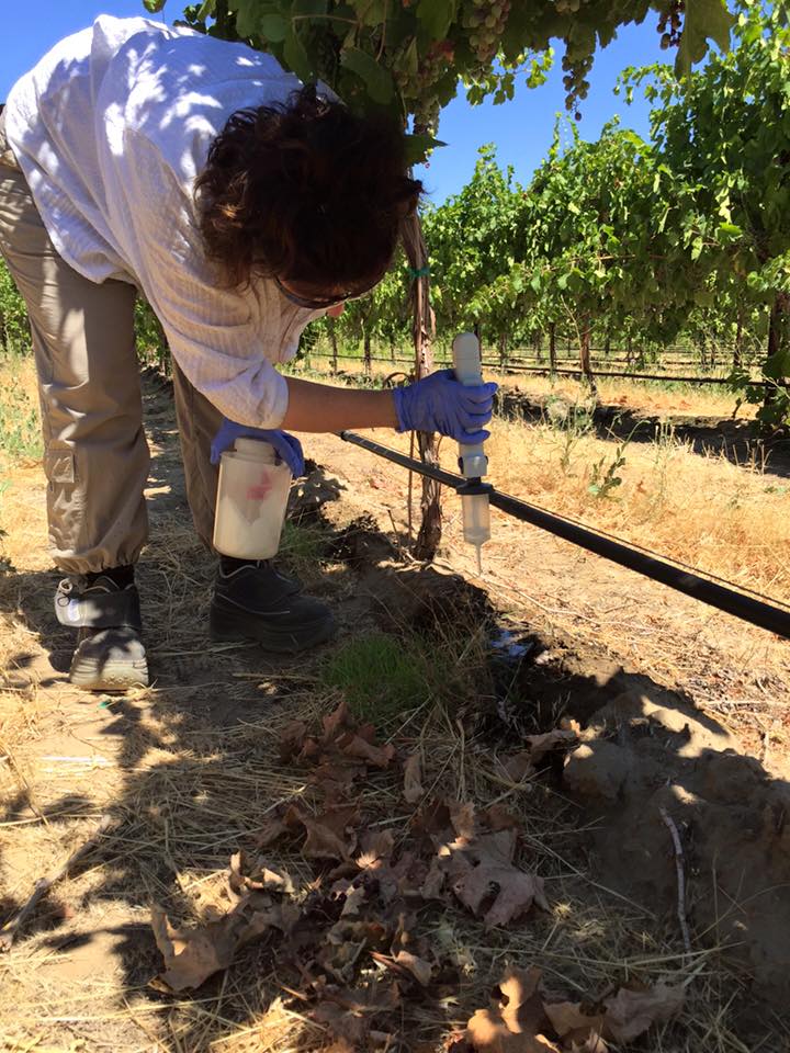
During the two growing seasons, we applied 0, 12, 25 or 37 lbs/A of P, divided across three applications. The timings of the applications were bloom, 1 month post bloom, and veraison, using sprays directly to the leaves (foliar application) or putting the P in with the irrigation water (Fig. 3).

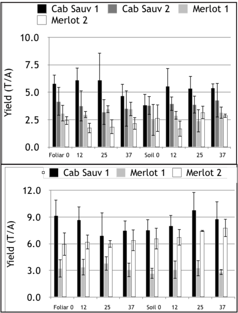
There were no differences in crop yield (Fig. 4) or quality factors (data not shown) between the fertilizer treatments in either year. Rather, yield reflected the difference in management of the vineyard blocks.
However, after two years of the same P fertilizer treatments, there were increases in leaf tissue P levels (Fig. 5) in the blocks that were low in P at the beginning of the experiment.

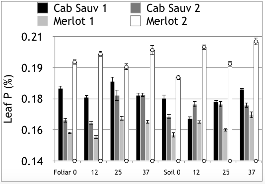
There were some slight differences in response between the two vineyards that were initially low in P, CS 2 and MR 1. In CS 2, leaf P reached the desired > 0.15% with all treatments, but was slightly higher with the foliar fertilizer applications than the soil applications. In MR 1, all treatments resulted in P that was at the desired level (Fig. 5). Overall these results suggest that either foliar or soil applied P can correct a P deficiency in vineyards. It should be noted that we did see leaf burning in the first growing season with the foliar treatments (even the lowest rates). Given that, since both soil and foliar-applied P are effective, and in one case (MR 1), soil-applied was effective at a lower rate, than soil-applied P is the better option. The results also suggest applying P at a rate of 25 lbs/A, split three times over the course of the growing season for two years will increase the leaf tissue P from deficient to sufficient.

Acknowledgments

This project was funded by the Washington State Grape and Wine Research Program, with additional support from WSU-ARC. Special thanks to Margaret McCoy, Jason Stout and Tanya Winkler for their assistance throughout the project.

References

1. Brady, N. C., and R. R. Weil. 2010. Elements of the nature and properties of soil, 3rd edition. Prentice Hall, San Francisco.
2. Davenport, J. R., and D. A. Horneck. 2011. Sampling guide and nutrient assessments for irrigated vineyards of the inland Pacific Northwest. Pacific Northwest Extension Publication #PNW622.
3. Marschner, H. 1986. Mineral nutrition of higher plants. Academic Press, San Diego.

Direct Root-Zone Irrigation in Vineyards

By Pete Jacoby, WSU Pullman

Water management is considered one of the most important means of achieving high quality wine grapes (1). Most wine grapes are irrigated by surface drip irrigation, considered to be an efficient means of watering compared to other contemporary methods.

However, application of water to the soil surface contributes to water losses from both evaporation to the atmosphere and use by weeds. Surface drip irrigation also tends to concentrate the roots in the upper soil profile, which dries rapidly during summer temperatures, requiring frequent irrigation applications to maintain vine health (2). Subsurface irrigation has been shown to be more water efficient than surface applied drip irrigation (3, 4). Unfortunately, use of buried driplines to deliver the water subsurface have been plagued with problems of soil clogging and gopher damage (5).

In 2014, research was initiated near Prosser, WA to deliver the water directly into the root zone via hard plastic tubes placed vertically into the soil. Tubes were placed from 1 to 4 feet below the soil surface in a mature planting of Concord juice grapes. Subsurface water delivery in the Concord grapes was reduced to 30 and 60 percent of full commercial rate applied as surface drip.

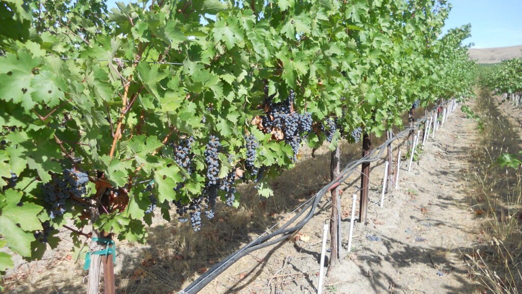
Two additional research sites were established in wine grape vineyards in early 2015 to deliver drip irrigation 1 to 3 deep (Fig. 1). For wine grapes, irrigation volumes were reduced to 15, 30 and 60 percent of the full commercial rate being applied as surface drip throughout the 2015 growing season.

Hypothetically, applying the water directly into the lower root zone should require a lower volume of water to be applied, owing to the elimination of evaporation and non-crop water use. This technique could also influence root architecture to change by growing deeper.

Likewise, root turnover could be expected to be reduced as roots become more densely concentrated in the portion of the soil profile that is less influenced by oscillating patterns of wetting and drying. If proven, the plant could become increasingly effective in carbon allocation, reserving more carbohydrates for fruit production. Watering intervals could be lengthened and deficit irrigation could be applied more strategically to regulate plant activity toward achievement of desired production and quality goals.

Preliminary results from the 2015 growing season are promising. Concord grape clusters were heavier and contained more berries in the subsurface irrigated plots than in the surface drip irrigation plots when irrigated at either of the reduced rates of water (30 or 60 percent of ET based water replacement).

In wine grapes, harvest production in subsurface irrigated plots was 70, 75, or 90 percent of that for the surface drip irrigated plots. However, the volume of water applied was 15, 30 or 60 percent, respectively, of that applied to the surface drip irrigated plots. Grapes tended to be smaller yet more numerous in the subsurface plots compared to the surface drip irrigated plots.

Next steps will include analytical assessment of wine grape phenolic compounds to determine what differences, if any, exist among the grapes produced under the differing levels of water stress. Both red and white wine grapes, as well as Concord grapes, are included in these trials underway on three separate site locations in the Yakima Valley.

References

1. Washington Association of Wine Grape Growers Sustainability Report
2. Stevens, R.M. and T. Douglas. 1994. Irrig. Sci. 12:181-186.
3. Bassoi, L.H., J.W. Hopmans, LA. Castro, C. Miranda, and J.A. Moura. 2003. Sci. Agricola 60(2):377-387.
4. Ayars, J.E., et. al. 1999. Agric. Water Manage. 42 (1):1-27.
5. Lamm, F.R., et. al. 2012. Trans. ASABE 55 (2):483-491.
6. Pocket Gophers #1 Enemy of subsurface Drip Irrigation in Western Alfalfa. Western Farm Press.

A Bubbly Perception – Complexity of Carbonation

By Kenneth McMahon (Graduate Student) and Carolyn Ross, WSU-Pullman, and Caleb Culver, Ste. Michelle Wine Estates

Carbonation, the tingling imparted by the presence of carbon dioxide, is an important sensory property in the acceptance of many beverages. While carbonation is influential in the acceptance of non-alcoholic beverages, it is also important in the identity of sparkling wine and contributes its characteristic effervescence [7]. Previous studies have developed vocabulary associated with the perception of carbonation in products such as milk [6], yogurt [10], soda [4], and sparkling water [1]. Despite the importance of carbonation to the acceptance of sparkling wine, less work has been performed on this product.

Sparkling wine contains dissolved carbon dioxide gas (CO₂) as a critical component [5]. By law, wines fall into the category of sparkling wines once the CO₂ levels reach ≥3.92 g CO₂/L (27 CFR 24.245). In sparkling wines, CO₂ can reach concentrations up to 11.8 g/L, but on average, CO₂ levels are near ~9 g/L [8]. The level of carbonation in the sparkling wine differs by sparkling wine style and standard of identity. Changes in wine processing steps may influence the sensory profile of the final sparkling wine, including its perceived carbonation.

Different sensory properties are associated with increased concentrations of CO₂. In a model beverage, the influence of CO₂ concentration on perceived sensory pain showed that more panelists reported perceived pain at 6.5 g CO₂/L compared to 3.2 g CO₂/L [2]. In white table wine, at concentrations of 1 g CO₂/L, the wine was described as prickly while at concentrations of 0.5 – 1.8 g CO₂/L, the wines were described as spritzy [9]

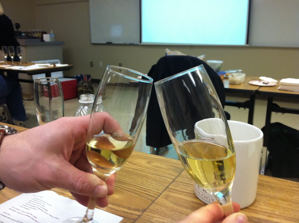
The influence of CO₂ on the sensory properties of the final wine, particularly mouthfeel, represent an area of great interest due to its anticipated influence on consumer acceptance. The overall objective of the study presented here was to determine the influence of wine processing, specifically the composition of the liqueur de tirage, on sensory properties of sparkling wines, with a focus on mouthfeel properties. This study also described the influence of these different carbonation levels on consumer perception.

In order to address our objective, eleven sparkling wine treatments were prepared by adding different concentrations of dextrose to a base wine. These dextrose concentrations were selected to result in wines of different CO₂ concentrations. As in the production of traditional sparkling wines, the wines underwent a secondary fermentation in bottle and were aged 9 months prior to evaluation. Once complete, the wines were analyzed for their chemical and sensory profiles. As intended, the wines differed in their carbonation concentrations and ranged from 0 – 7.5 g/L CO₂ based on the concentration of dextrose that was added.

The profile of these wines was characterized using a trained panel. Panelists (n=11) were trained over 15 one-hour sessions on the tasting procedure. Sample handling by the panelist, sample pouring and preparation were carefully controlled to minimize CO₂ loss over time. Using standards, the panelists were trained to recognize the mouthfeel attributes of bite, burn, carbonation/bubble pain, foamy, numbing, after-numbing, pressure, prickly, and tingly. Specific taste, flavor and aroma attributes were also analyzed. These trained panelists were also trained to evaluate the sparkling wines samples using a “temporal check all that apply” (TCATA) methodology. This method allowed the panelists to check and uncheck attributes as they are perceived, capturing the changes in perception over time.

For the consumer evaluations, a paired comparison test was used, with wine pairs presented to each panelist for the identification of the sample with the higher intensity of a particular attribute. Six paired comparison tests were conducted in which each CO₂ concentration (0, 1.2, 2.0, 4.0, 5.8, and 7.5 g CO₂/L) was compared to the control sparkling wine (0 g CO₂/L). For each pair, consumers were required to evaluate both samples and indicate which sample of the pair had a greater intensity of the mouthfeel attributes of carbonation and “bite”, along with identifying which sample had a more sour taste. The experiment was repeated on a second day.

Due to the influence of temperature on CO₂ perception, for both the trained and consumer panels, all wines were maintained and presented at 40°F. At least two bottles per treatment were opened so as to avoid significant CO₂ losses from the kinetics of pouring and wait time.

Results

The trained panel data analysis revealed that mouthfeel attributes were the main drivers of differences among the wine treatments, with 95.3% of the variability observed among the wine treatments being attributed to mouthfeel attributes. The trained panel data analysis also showed the separation of the sparkling wine treatments based on their carbonation levels. Specifically, the wines containing the highest concentrations of CO2 (4.6 – 7.5 g /L CO₂) were defined by the highest intensities of the mouthfeel attributes of pressure, bite, foamy, and prickly. The sparkling wines with lower carbonation levels (0 g /L CO₂ to 3.1 g /L CO₂) were less defined by these mouthfeel attributes.

Given the influence of mouthfeel on the separation of these samples, subsequent work profiled the complexity of carbonation perception. For this second trained panel, 13 panelists received training on the TCATA method and following this training, evaluated wines using the TCATA protocol. This protocol instructed the panelists to sip the entire contents of the wine, immediately begin checking/unchecking attributes as they perceived them, after 10 sec were prompted to expectorate, and continue the evaluation through 2 min.

TCATA results indicated that mouthfeel attributes were separated into two time periods, those that were perceived ‘early’ (peaked at ~8 sec) and those that were perceived ‘later’ (peaked at ~24 sec) in the evaluation period. During this early phase, the attributes of bite/burn, carbonation/bubble pain, foamy, and prickly/pressure were mentioned more frequently to describe the sample. After 8 sec, the sample was more frequently described by the attributes of numbing, tingly, bitter, and sour.

Significant differences were observed among the wine treatments. Bite/burn, an attribute perceived in the ‘early’ portion of the evaluation, peaked at ~8 sec and was cited at different frequencies among the four sparkling wines containing 0, 1.2, 4.0, and 7.5 g/L CO_2. After this ‘early’ perception time had passed, wine treatments were not significantly different in the proportion of citations for this attribute. In contrast, during the ‘late’ perception time (peaked at ~24 sec), the citation of ‘tingly’ was significantly different among the four sparkling wines containing 0, 1.2, 4.0, and 7.5 g/L CO₂. The different patterns in citations of different mouthfeel attributes during the course of evaluation demonstrated how TCATA could provide information regarding the dynamic nature of carbonation perception, information that would have been missed by the traditional trained panel.

Consumer Panel: Paired comparison testing was conducted to determine if consumers were able to distinguish between a control wine (containing 0 g CO₂/L) and a sparkling wine treatment containing 1.2, 2.0, 4.0, 5.8 or 7.5 CO₂/L. The mouthfeel attributes of carbonation (“which wine is more carbonated?”) and bite (“which wine has more bite?”) were examined. For both attributes, when the control wine (0 g CO₂/L) was compared to itself (blind control) or compared to the sparkling wine containing 1.2 g CO₂/L, no significant differences in any attributes were found. However, when the control wine was compared to 2.0 g CO₂/L, more consumers selected the treatment wine as being more “carbonated” and having more “bite” (p≤0.05). As the CO₂ concentration increased to 4.0, 5.8 and 7.5 g CO₂/L., the number of consumers selecting the treatment wine as being more “carbonated” and having more “bite” increased and then plateaued (p≤0.001).

These results suggest that the minimum concentration of CO₂ (g/L) required for consumers to distinguish between sparkling wine treatments for the sensory attributes of carbonation and “bite” was >1.2 g CO₂/L. These findings support a previous study in which Harper and McDaniel [3] reported that a trained panel reported a greater mouthfeel perception of “bite” in carbonated water as CO₂ increased in concentration from 0 to 0.9 g CO₂/L. The results also suggest that differences exist in panelist sensitivity to carbon dioxide. Beyond the comparison of the base wine to 4.0 g CO₂/L, the number of consumers identifying the treatment with higher CO₂ concentration did not appreciably change.

Conclusions

Using trained panelists, sparkling wines of varying carbonation levels were evaluated using a traditional trained panel and a trained panel using TCATA methodology, each of which generated a detailed profile of carbonation perception. The trained panel showed a positive correlation among the intensity of different mouthfeel attributes and CO₂ concentration. TCATA provided the dynamic profile of carbonation of sparkling wines and shed light on the complexity and temporality of effervescence. Specifically, during this early phase (up to 8 sec after placing the sample in-mouth) of effervescence perception, the attributes of bite/burn, carbonation/bubble pain, foamy, and prickly/pressure were mentioned more frequently to describe the sample. Around 24 sec, persistent attributes were cited more frequently, including numbing, tingly, and the tastes of bitterness and sourness.

In the sensory evaluation of these wines by consumers, results showed that at CO₂ concentrations >1.2 g CO₂/L, consumers identified the CO₂ wine was having more “bite” and carbonation than the control wine with no carbonation. The results of this study provide sparkling winemakers and manufacturers of other carbonated products, such as beer, soda, and water, insight into the influence of CO₂ on consumer perception.

References

1. Dessirier, J.M., et. al. 2001. Chemical Senses, 26(6), 639-643.
2. Green, B.G. 1992. Chemical Senses, 17(4), 435-450.
3. Harper, S.J., & McDaniel, M.R. 1993. Journal of Food Science, 58, 893-897.
4. Kappes S.M., Schmidt S.J., & Lee S.Y. 2007. Journal of Food Science, 72,S1–S11.
5. Le Barbé, E. 2014. (Unpublished master’s thesis). Kansas State University, Manhattan, KS.
6. Lederer, C.L., Bodyfelt, F.W., & McDaniel, M.R. 1991. Journal of Dairy Science, 74(7), 2100-2108.
7. Liger-Belair, G., et. al. 2007. Journal of Agricultural and Food Chemistry, 55(3), 882-888.
8. Liger-Belair, G., Polidori, G., & Jeandet P. 2008. Chemical Society Reviews, 37(11), 2490-2511.
9. Peynaud, E. 1983. The taste of wine: the art and science of wine appreciation. San Francisco: The Wine Appreciation Guild, Ltd.
10. Wright, A.O., Ogden, L.V., & Eggett, D.L. 2003. Journal of Food Science, 68(1), 378-381.

Investigating Brett in Vineyards & Oak Barrels

By Zach Cartwright (Graduate Student) and Charles Edwards, WSU Pullman

Spoilage by the yeast Brettanomyces bruxellensis poses a concern, if not a major threat, to red wine quality. It can produce aromas described as ‘horse sweat,’ ‘animal,’ ‘stable,’ and ‘medicinal’ that taint a finished wine’s bouquet. Brettanomyces is also known to produce ‘vinegar’, ‘nail polish remover’, ‘mousy’ and ‘rancid’ odors through the production of various secondary metabolites.

In order to prevent these defects and widespread contaminations, effective control measures for this microorganism are needed for the wine industry. The Edwards lab at Washington State University is helping to accomplish this by answering questions about Brettanomyces’ survival in vineyards and oak barrels.
While isolations of this yeast from grapes have been reported, concrete evidence of its long-term existence in vineyards is inadequate. But how does it get into the vineyard to begin with? One common practice of interest is the spreading of winery waste products throughout vineyards. While pomace may be beneficial for grape development, it may be infected with low populations of Brettanomyces (the yeast can survive alcoholic fermentation).

Our laboratory is currently tracking the survival of Brettanomyces in several types of pomace samples in Pacific Northwest vineyards. The information from these studies will demonstrate how populations of the yeast change seasonally in different outdoor settings and give better insight into whether this vineyard practice is leading to in-vineyard contamination.

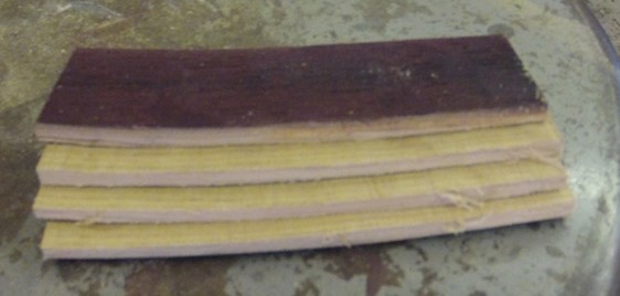
Oak barrels are also considered one of the most common sources for contamination (Fig. 1). However, penetration of the yeast in oak pores have not been well defined nor studied. Understanding how infections differ with respect to oak type, toasting level and stave location within a barrel would allow for better cleaning recommendations on a barrel-to-barrel basis. Currently, we are conducting trials using steam and hot water treatments as these methods are used by the wine industry. This information will give winemakers better guidelines to follow when decontaminating infected oak barrels and provide assurance for use of the barrels during future harvests.

By exploring Brettanomyces survival in vineyards and oak barrels, our laboratory is continuing its goal of helping to develop new and effective control measures for this microorganism. The impact on wine quality and economic loss cause by Brettanomyces make it a top priority for our team. Findings from our lab have guided the wine industry in the past regarding spoilage prevention, and these studies hope to do the same.

Building References: Viticulture Publications

On-Farm Vineyard Trials: A Growers Guide (#EM098)

On-farm research offers many opportunities to understand the effectiveness of various management practices and products. However, how these trials are designed can alter the observed results.

This guide summarizes the concepts of experimental design and how those concepts are important in conducting field trials and understanding their results. It also describes specific examples of trial design and explains how to collect data relevant to vineyard research. Simple statistical tests that are used to help interpret results are also explained.

Download the On-Farm Vineyard Trials: A Growers Guide.

Viticulture publications — En Español!

Funded by NIFA-AFRI-CPPM, several Viticulture Extension publications have been translated into Spanish:

• Oídio de la uva para producción comercial en el este de Washington: Biología y manejo de la enfermedad – EM058ES
• Evaluación y manejo del daño por frío en los viñedos de Washington – EM042ES
• Conceptos básicos de riego para los viñedos del este de Washington – EM061ES
• Estimación del rendimiento del viñedo – EM086ES